Saturday, June 22, 2019

Analyzing MSFT Financial Data using AlphaVantage and Google Colab

In today's world, it's very easy to analyze data sets online, including financial data. This article shows how to compute standard statistical properties of a financial data set, like linear approximation and standard deviation. The example is using python based jupyter notebook, shared through Google Colab.

Here's a Jupyter Notebook, which can be used for this exercise.

First, we start by creating an API key in AlphaVantage.


Next, we can display a downloaded financial dataset, which corresponds to MSFT historical data.

After this step, we run statistical analysis of dataset using Python stats library.

from scipy import stats

slope, intercept, r_value, p_value, std_err = stats.linregress(x, y)


Then, we can display the resulting data using Matplotlib. The chart will be displayed in the result window of Jupyter Notebook:


Google Research Colab is a very popular and simple tool for running all sorts of data set analysis tasks. This also includes deep learning using tensorflow library. It is a step forward into simplifying data analysis in the research community.


Sunday, April 16, 2017

Landing on The Moon using AI Bot

Recently I was playing around with OpenAI Gym and Keras Reinforcement Learning library (keras-rl). I was able to train an AI Agent for a task of landing on the Moon. 

OpenAI Gym provides all sorts of different environments to explore using AI bots. One of them is lunar lander, which I'll focus on here. 
Keras on the other hand is a high level library built on top of TensorFlow (or Theano). It provides mechanisms for constructing deep learning models easily. 

Creating a new environment using OpenAI Gym is as easy as this:

env = gym.make('LunarLander-v2')

Here's how you can add video recorder of progress during training:

env = gym.wrappers.Monitor(env, 
                           'recording', 
                           resume=True, 
                           video_callable=lambda count: count % record_video_every == 0
                           )

The model itself is quite simple DQN Agent with LinearAnnealedPolicy. The most important layer is Dense 512 neuron internal layer. It's responsible for understanding of the current situation during landing. Next small, dense layer on top of it is responsible for final decisions related to lunar lander actions (steering the engines).

Here's how it can be instantiated:

model = Sequential()
model.add(Flatten(input_shape=(1,) + env.observation_space.shape))
model.add(Dense(512))
model.add(Activation('relu'))
model.add(Dense(nb_actions))
model.add(Activation('linear'))
print(model.summary())

memory = SequentialMemory(limit=1000000, window_length=WINDOW_LENGTH)

policy = LinearAnnealedPolicy(EpsGreedyQPolicy(), attr='eps', value_max=1., value_min=.1, value_test=.05, nb_steps=1000000)

dqn = DQNAgent(model=model, nb_actions=nb_actions, policy=policy, memory=memory, nb_steps_warmup=50000, gamma=.99, target_model_update=10000, train_interval=4, delta_clip=1.)

dqn.compile(Adam(lr=.00025), metrics=['mae'])


Here's a summary of the model:

Layer (type)                     Output Shape          Param #     Connected to                 7    
flatten_1 (Flatten)              (None, 8)             0           flatten_input_1[0][0]            
dense_1 (Dense)                  (None, 512)           4608        flatten_1[0][0]                  
activation_1 (Activation)        (None, 512)           0           dense_1[0][0]                    
dense_2 (Dense)                  (None, 4)             2052        activation_1[0][0]               
activation_2 (Activation)        (None, 4)             0           dense_2[0][0]                    

Total params: 6,660
Trainable params: 6,660
Non-trainable params: 0


Training can take a lot of time. In this example I used 3.5 million steps.
The outcome gives quite reasonable behavior for lunar lander.
Note that depending on environment, learning can take less time (if environement is not very tricky). In this case I found that difficulties are related to sensitivity of the last phase of landing (touch down). It took some time for the model to figure this part out.

As a side note, OpenAI provides lunar lander Agent using optimal trajectory. In this example, the Agent polls environment to figure out actions that give highest output of Q function. 


Saturday, March 18, 2017

Classifying Dogs vs Cats on a Regular Laptop with 2GB GPU and 90% Accuracy


Machine learning ecosystem has evolved a lot during recent years.
I am amazed that I could run a very sophisticated experiment of classifying dogs vs cats with 90% accuracy on my regular laptop laptop.
It has 2GB NVidia GPU card and 8GB RAM.
Just in 2012 the state of art result of the dogs vs cats classification was 80%.

I ran it based on an excellent course provided by fast.ai (http://course.fast.ai/).
The competition is organized by Kaggle:
https://www.kaggle.com/c/dogs-vs-cats-redux-kernels-edition

Here's an overview of the approach taken to achieve 90% accuracy.
First, retrieve a publicly available model VGG16, which was prepared by scientists for image recognition competition (for ImageNet). Then remove last layer out of it and replace with Yes / No layer for recognizing cats vs dogs. The remaining layers were set as non trainable. Then run learning process for such model.

The main libraries used here are Keras with Tensorflow backend.

Full code is available on fast.ai website. Here in an overview of the most important parts.
Training code:

import tensorflow as tf
from keras.backend.tensorflow_backend import set_session
config = tf.ConfigProto()
config.allow_soft_placement=True
config.log_device_placement=True
set_session(tf.Session(config=config))

# Import our class, and instantiate
import vgg16; reload(vgg16)
from vgg16 import Vgg16
vgg = Vgg16()

batch_size=16
path = "data/dogscats/"
#path = "data/dogscats/sample/"
batches = vgg.get_batches(path+'train', batch_size=batch_size)
val_batches = vgg.get_batches(path+'valid', batch_size=batch_size)
vgg.finetune(batches)
vgg.fit(batches, val_batches, nb_epoch=1)
vgg.model.save('vgg2.h5')

The code uses vgg.finetune call to update the last layer of the model. Here's how it looks like:

model = self.model
        model.pop()
        for layer in model.layers: layer.trainable=False
        model.add(Dense(num, activation='softmax'))

Next, it trains model using vgg.fit call and saves result to vgg2.h5 file. 

I had to put a few tweaks to the model related to device placement for Tensorflow so it could fit in GPU memory. The last few layers were placed on CPU. Here's the code:

      model = self.model = Sequential()
        model.add(Lambda(vgg_preprocess, input_shape=(3,224,224), output_shape=(3,224,224)))

        with tf.device('/gpu:0'):
            self.ConvBlock(2, 64)
            self.ConvBlock(2, 128)
            self.ConvBlock(3, 256)
            self.ConvBlock(3, 512)
            self.ConvBlock(3, 512)

        with tf.device('/cpu:0'):
            model.add(Flatten())
            self.FCBlock()
            self.FCBlock()
            model.add(Dense(1000, activation='softmax'))

        fname = 'vgg16.h5'
        model.load_weights(get_file(fname, self.FILE_PATH+fname, cache_subdir='models'))


Here's the result of a learning process:

23000/23000 [==============================] - 2103s - loss: 0.5482 - acc: 0.8676 - val_loss: 0.4194 - val_acc: 0.9060

The training process completed in 35 minutes with 90% accuracy on validation set. 

I'm very positively surprised that such powerful machine learning tools are available these days and are runnable on regular computers. Moreover the approach presented by fast.ai is very interesting and resembles natural evolution of intelligence by adding new layers. 

Sunday, March 13, 2016

Learning Sine Function Using Neural Network


Recently I stumbled upon an excellent demo of a 2 layer neural network written by Florian Muellerklein: https://github.com/FlorianMuellerklein/Machine-Learning.

It is written in Python using numpy and focuses on digit recognition based on sklearn dataset.
I decided to play around with it and add visualization for learning process of a sine function.
I used matplotlib for creating an animation.

The neural network implementation is typical. It uses standard gradient descent procedure with some optimizations like momentum and regularization (also random initialization).
If you are interested in understanding how exactly gradient descent works, I highly recommend an article from Matt Mazur: http://mattmazur.com/2015/03/17/a-step-by-step-backpropagation-example.

The network architecture I used was following:

  • 1 input neuron (x parameter of sine function)
  • 60 hidden neurons
  • 1 output value (the function result)

Here is a link to source code: https://github.com/rafalrusin/Machine-Learning/tree/master2

It converges pretty well. Here's an animation showing convergence of sine function during consecutive learning iterations (10 learing iterations per frame):


Machine Learning is a very fascinating domain that has been emerging rapidly over recent years, mainly in visual object recognition. I hope that it keeps this pace in future (or even exceeds it!).

Saturday, May 16, 2015

Asymptotic Benchmark in Java

Most of the time when we analyze performance of different programs, we use Big O Notation and run performance tests for a single input size N, which measures execution time.

Both of these methods have disadvantages.
Big O Notation is theoretical (has no code verification).
Time based performance tests are not very reliable (it's hard to make assertions on them) and don't show the actual asymptotic function behind the programs.

Here I present a slightly different approach, which is a combination of those 2 techniques.
It uses explicit instruction counting, samples programs for different input sizes and tries to guess asymptotic function behind them.
It also plots the result as a chart using HTML and Google Visualization JavaScript Library.

Note that it's more of a toy for visualization than something one could use in the industry for real world projects.

First we start by implementing an example program (Binary Counter), which we want to measure. It'll extend a base class Benchmark, which looks like this (full source code is available on github: https://github.com/rafalrusin/abench):

public abstract class Benchmark {
    private int instructionCount = 0;

    protected void incrementInstructionCount() {
        instructionCount++;
    }

    public void resetInstructionCount() {
        instructionCount = 0;
    }

    public int getInstructionCount() {
        return instructionCount;
    }

    protected abstract Object run(int n);
}

It has abstact method "run", which takes input size as argument. This will be provided by the benchmark framework for different executions. 
Binary Counter implementation looks like this:

public class BinaryCounter extends Benchmark {
    @Override
    protected Object run(int n) {
        int[] counter = new int[64];
        for (int i = 0; i < n; i++) {
            int p = 0;
            while (counter[p] == 1) {
                counter[p++] = 0;
                incrementInstructionCount();
            }
            counter[p] = 1;
            incrementInstructionCount();
        }
        return counter;
    }
}

It is a 64 bit binary counter, which starts from 0 and increments values N times by one. Theoretically it should run in O(n) time. We'll verify that. 

We need to run it through the framework using following code:

public class Main {
    public static void main(String[] args) {
        BenchmarkRunner benchmarkRunner = new BenchmarkRunner();
        benchmarkRunner.addFormatter(new TextResultFormatter(new PrintWriter(System.out)));
        benchmarkRunner.addFormatter(new HtmlResultFormatter(new File("out")));

        for (Benchmark benchmark : new Benchmark[]{
                new BinaryCounter(),
                ...
                ) {
            benchmarkRunner.run(benchmark, 1);
        }
    }

Here's the chart generated for Binary Counter along with guessed function behind it:


In this case the guessed function is linear, which is what we expected. For input size of 5.6 millions, the instruction count was 11 million.

The guessing process is an iteration over all samples and optimization of Mean Squared Error.
It is implemented in BenchmarkRunner class. 
You can add more functions by extending Function interface. Here's an example of N log N function:

public class NLogNFunction implements Function {
    @Override
    public float eval(float x) {
        return (float) (Math.log(x) * x);
    }
}

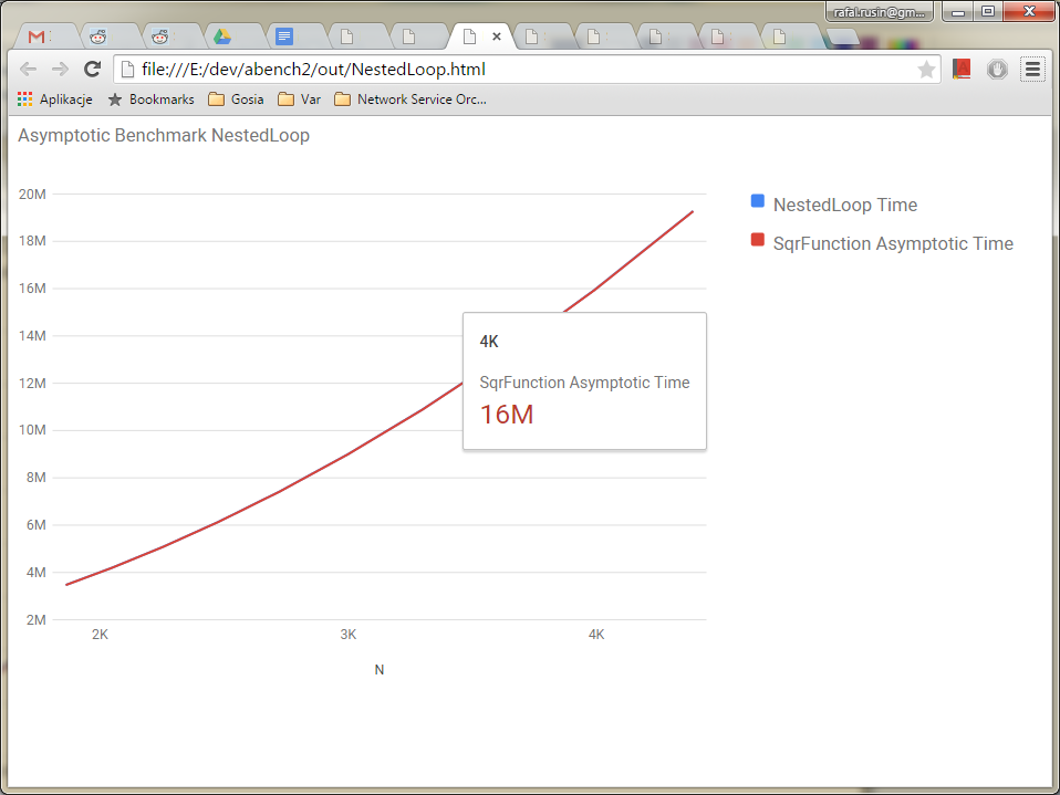
Here's some more benchmarks: MergeSort (expected asymptotic function is N log N) and NestedLoop (N^2). 


Implementing reliable performance tests is not a very well solved problem today. I think that the idea of instruction counting is something one can try to use in real world projects. It can be used for testing performance of isolated chunks of code, within unit tests, and can give predictable results. 

Sunday, November 23, 2014

Handling requests Asynchronously in Java using Jersey 2.13 and Glassfish 4.1


In recent Jersey release 2.x, there is a new API for async request processing. It includes an excellent example server-async-standalone-webapp.
In this article, I'll show how to run it and the results we can get by leveraging async processing.

First, we need to download Glassfish 4.1 Web profile (https://glassfish.java.net/download.html).
Then start it using command:

./asadmin start-domain

Next, we need to download Jersey examples bundle from https://jersey.java.net/download.html and compile server-async-standalone example by running 'mvn package'.

Then we can deploy it using following command:

./asadmin deploy <path>/jersey/examples/server-async-standalone/webapp/target/server-async-standalone-webapp.war

Now we are ready to login to Glassfish Admin Console (localhost 4848) and see the status of deployed application:


Now we're ready to run a client GUI application, which allows us to run tests against server. Go to 'server-async-standalone/client' and run 'mvn exec:java'. 
The application looks like below. I ran sync vs async test on 100 requests and got response times improved from 20 secs to 1.2 secs. 

Sync

Async


The code is following for sync:

    @GET
    @Path("sync/{echo}")
    public String syncEcho(@PathParam("echo") final String echo) {
        try {
            Thread.sleep(SLEEP_TIME_IN_MILLIS);
        } catch (final InterruptedException ex) {
            throw new ServiceUnavailableException();
        }
        return echo;

    }

And for async:

private static final ExecutorService TASK_EXECUTOR = Executors.newCachedThreadPool();
...
    @GET
    @Path("async/{echo}")
    public void asyncEcho(@PathParam("echo") final String echo, @Suspended final AsyncResponse ar) {
        TASK_EXECUTOR.submit(new Runnable() {

            @Override
            public void run() {
                try {
                    Thread.sleep(SLEEP_TIME_IN_MILLIS);
                } catch (final InterruptedException ex) {
                    ar.cancel();
                }
                ar.resume(echo);
            }
        });
    }

Note that in Async example, the number of background threads is unbounded (TASK_EXECUTOR is a cached thread pool without limit). So in reality it won't improve the amount of resources (threads) consumed by server in Aync mode. 
In Sync mode, the threads hold http executor. The default number of http worker threads in Glassfish is 5. This explains why we get response time around 20 secs for 100 requests. 

"http-listener-1(4)" daemon prio=6 tid=0x000000000cc7d000 nid=0xcf8 waiting on condition [0x00000000110ad000]
   java.lang.Thread.State: TIMED_WAITING (sleeping)
at java.lang.Thread.sleep(Native Method)
at org.glassfish.jersey.examples.server.async.LongRunningEchoResource.syncEcho(LongRunningEchoResource.java:77)
at sun.reflect.GeneratedMethodAccessor437.invoke(Unknown Source)
...

Note that this is just an example, which illustrates how to enable Async processing. In real world scenarios there can be a third party service, which can be invoked using Jersey Client on the server side. If that service slows down, then the whole http thread pool on the server side can be exhausted and prevent other requests from getting processed. 
The suggested solution in this case would be to switch to Async Jersey Client and Async service implementation. 

Async server processing can also help in case where there is a lot of slow clients. For example 20k mobile clients, who send payloads in chunks with 1 second delays. This scenario can easily bring down Sync server side implementations.

Async processing is gaining momentum on server side nowadays. There are multiple technologies, 
which enable it. Among them are NodeJS, Netty, Akka and Play Framework. Jersey Async processing is one of them.  


Saturday, July 5, 2014

Implementing a Distributed Counter Service Using Hazelcast, Jersey 2 and Guice

Modern web services are often required to scale horizontally in order to handle growing load.
Here I present an example distributed Counter service, which uses modern technology stack consisting of Hazelcast, Jersey 2 and Guice.

The sample is based on an excellent example posted by Piersy and can be downloaded from here:
http://github.com/rafalrusin/jersey2-guice-example-with-test

The counter is just a shared value across all participating nodes within a cluster. All nodes can query for data and increase it's value by specified delta. Note that Hazelcast handles synchronization within distributed environment. In order to update the state atomically, we use Hazelcast EntryProcessor.

@Singleton
public class CounterService {

    public int increase(final int delta) {
        return (Integer) map.executeOnKey("counterKey", new CounterEntryProcessor(delta));
    }
}

public class CounterEntryProcessor implements EntryProcessor<String, Integer>, EntryBackupProcessor<String, Integer> {
    private final int delta;

    public CounterEntryProcessor(int delta) {
        this.delta = delta;
    }

    @Override
    public Integer process(Map.Entry<String, Integer> entry) {
        int newValue = entry.getValue() + delta;
        entry.setValue(newValue);
        return newValue;
    }
}

The service is just a Guice Singleton. It has an operation called 'increase', which takes a delta and creates EntryProcessor job for Hazelcast to submit to a node, which owns the value at the time and will update it atomically.
Hazelcast is a library, which implements Java Collections in distributed fashion. It handles replication, cluster membership and distributed locking.

Web service is a simple JAXRS REST Resource. Following code invokes Guice service layer from Resouce implementation:

@RequestScoped
@Path("counter")
public class CounterResource {

    private CounterService service;

    @Inject
    public CounterResource(CounterService service) {
        this.service = service;
    }

    @POST
    @Consumes(MediaType.TEXT_PLAIN)
    @Produces(MediaType.TEXT_PLAIN)
    public String increase(String delta) {
        return "" + service.increase(Integer.parseInt(delta));
    }
}

We also have a test case, which invokes the whole stack and does a request to the service. The whole stack is very lightweight. In runs on Jersey with Embedded Tomcat. The test case completes within a few seconds.

In order to run the example, you need to build distribution first (run dist.sh), then start nodes in separate shells and invoke curl POST requests to manipulate counter state. Here's a sample interaction:

./run.sh 8090
./run.sh 8092
...
Jul 05, 2014 10:20:06 AM com.hazelcast.cluster.ClusterService
INFO: [10.0.0.12]:5702 [dev] [3.2.3]

Members [2] {
        Member [10.0.0.12]:5701
        Member [10.0.0.12]:5702 this
}

Jul 05, 2014 10:20:08 AM com.hazelcast.core.LifecycleService
INFO: [10.0.0.12]:5702 [dev] [3.2.3] Address[10.0.0.12]:5702 is STARTED
...

$ curl -d '1' -H 'Content-Type: text/plain;' http://localhost:8092/webapp/api/counter
22
$ curl -d '1' -H 'Content-Type: text/plain;' http://localhost:8090/webapp/api/counter
23
$ curl -d '5' -H 'Content-Type: text/plain;' http://localhost:8090/webapp/api/counter
28

I think that Hazelcast is a very good step forward into distributed computing. For an every day programmer, it's a set of primitives to manipulate in order to implement a distributed system. It is very easy to integrate it into existing project, which could be either JavaEE or standalone app.